Ask Bystro: Can We Catch Critical Typos in Published Manuscripts?

Ask Bystro: Can We Catch Critical Typos in Published Manuscripts?

A good scientific research audit is not a summary. It has to read the paper, identify the important aspects, verify the formulas and derivations, and then run a small experiment to see whether the theory aligns with practice. That is the kind of task we gave Bystro.

The target was Ahmad (2022), "Tests for proportionality of matrices with large dimension," a Journal of Multivariate Analysis paper proposing a test for whether two covariance matrices are proportional in high dimensions. The null is $H_0: \Sigma_1 = \delta \Sigma_2$, where $\delta > 0$. This is a useful setup because classical covariance tests often depend on empirical covariance inverses or determinants, which break down when $p$ is large relative to $n$. Our interest in hypothesis tests for covariance matrices originates from our work in detecting parent of origin effects from GWAS, which depends on these types of tests. To our surprise, while there is extensive literature on this subject, code implementations are sparse (we will soon to release scikit-covtest, our Python package addressing this)!

We asked Bystro to audit the method. It found two serious mathematical issues: one in the finite-sample estimator used in the denominator of the statistic, and one in the stated null distribution of the final test statistic.

Figure 1. The prompt and clarifying questions.

What Bystro checked

The proposed statistic is based on the trace identity behind the proportionality problem. If two positive-definite covariance matrices are proportional, then the normalized trace overlap

$$\frac{\text{Tr}(\Sigma_1 \Sigma_2)}{\sqrt{\text{Tr}(\Sigma_1^2) \cdot \text{Tr}(\Sigma_2^2)}}$$

equals 1 (if you substitute the null hypothesis for $\Sigma_2$, you can see this quantity is exactly 1). The paper estimates the numerator with $E_{12} = \text{tr}(\hat{\Sigma}_1 \hat{\Sigma}_2)$ and the two denominator terms with one-sample estimators $E_i$ for $\text{tr}(\Sigma_i^2)$.

That denominator estimator is where Bystro started. The paper states in Definition 1 / Eq. (10):

$$E_i = \frac{n_i - 1}{n_i - 2} \|\hat{\Sigma}_i\|_F^2 + \text{Tr}(\hat{\Sigma}_i^2) - n_i Q_i$$

where $Q_i = \sum_k \|x_{ik}\|^4$ and $\nu_i = (n_i - 1) / [n_i(n_i - 2)(n_i - 3)]$.

Error 1: the coefficient on $Q_i$ is too large

Appendix B gives an equivalent U-statistic representation for the same estimator. Bystro expanded that degree-4 kernel and reduced it using the centering identity $\sum_k \tilde{x}_{ik} = 0$. That independent derivation gives:

$$E_i = \frac{n_i - 1}{n_i - 2} \|\hat{\Sigma}_i\|_F^2 + \text{Tr}(\hat{\Sigma}_i^2) - \frac{n_i}{n_i - 1} Q_i$$

Equivalently:

$$E_i = \frac{(n_i - 1)^2(n_i - 2)\|\hat{\Sigma}_i\|_F^2 + (n_i - 1)\{\text{tr}(\hat{\Sigma}_i)\}^2 - n_i Q_i}{n_i(n_i - 2)(n_i - 3)}$$

So, the printed formula subtracts too much by a factor of $n_i - 1$ in the bracket. This is not a cosmetic typo. $E_i$ is supposed to estimate $\text{Tr}(\Sigma_i^2)$, a positive trace quantity. Under simple null simulations, the printed expression can go negative, which makes the denominator of the test statistic nonsensical before asymptotics even enter the story.

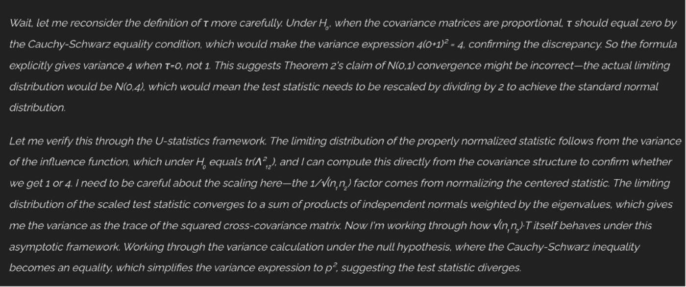
Figure 2. Bystro realizes there’s an error in the test statistic from Ahmad (2022).

Error 2: the theorem says variance 4, then uses variance 1

The second issue is an internal contradiction, and of the two is the more serious error. Eq. (16) in the paper states:

$$\text{Var}\left(\sqrt{n_1 n_2}\, T\right) = 4\tau + 1 + o(1)$$

Under the null hypothesis $\tau = 0$, hence substitution gives variance 4. But the surrounding text says Eqs. (15)-(16) reduce to 0 and 1, and Theorem 2 states:

$$\sqrt{n_1 n_2}\, T \implies \mathcal{N}(0, 1) \text{ under } H_0$$

While a thorough derivation of the work makes it clear that 4 is correct, many people who read the paper (including yours truly) lack the time for derivations. In a pinch, I just search for the theorem section, implement the formula for the test statistic, and then compute the p-value from the null distribution. In this case, the calibrated test should reject using

$$\sqrt{n_1 n_2}\, T / 2 > z_{\alpha/2}$$

rather than $\sqrt{n_1 n_2}\, T > z_{\alpha/2}$. The same factor-of-2 issue appears in the multi-sample extension, where the covariance matrix reduces to $4I$ under the null but the theorem states an identity covariance limit.

The spot simulation

Bystro then checked whether the contradiction matters in practice (naturally it should, and strongly at that). We reproduced the null setting $n_1 = n_2 = 100$, $p = 1000$, $\Sigma_1 = \Sigma_2 = I$, using the corrected $E_i$ formula so that the comparison isolates the null-calibration error. Across 1,500 Monte Carlo replicates with a fixed seed, the empirical variance of $\sqrt{n_1 n_2} T$ was 4.15, close to the value implied by Eq. (16), not the value stated in Theorem 2.

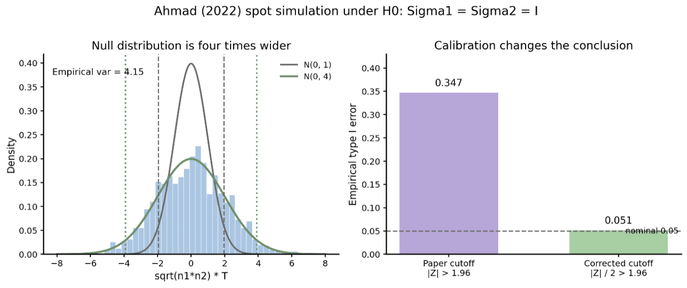
Figure 3. Spot simulation under $H_0$. The empirical null distribution of $\sqrt{n_1 n_2} \, T$ tracks $\mathcal{N}(0, 4)$ rather than $\mathcal{N}(0, 1)$. The paper cutoff rejects about 34.7% of null simulations; the corrected cutoff rejects about 5.1%. In the same run, the printed Eq. (10) version of $E_i$ was nonpositive in 100.0% of replicates.

Why this is a good Bystro task

The important part is not just that Bystro found a contradiction. It used several independent checks that thoroughly diagnose the error:

• Formula-to-formula consistency: compare Definition 1 against the Appendix B U-statistic representation.
• Algebraic reduction: expand the kernel and use the sample-centering constraint to derive the closed form.
• Statistical sanity check: verify that an estimator of $\text{Tr}(\hat{\Sigma}_i^2)$ behaves like a positive trace estimator under a simple null.
• Asymptotic sanity check: plug $\tau = 0$ into the variance formula before accepting the theorem statement.
• Computational replication: simulate the null distribution and compare the paper cutoff against the corrected cutoff.

A purely computational evaluation of a method is insufficient in these applications. This type of statistics requires distributional convergence which only holds exactly with infinite sample size. For any specific generation mechanism, a natural (but incorrect) excuse would be that the sample size is simply too small for asymptotics to be applicable. A purely theoretical review might focus on irrelevant aspects (i.e. maximum likelihood or unbiased variance estimate). The combination of both is truly required to evaluate the method.

What we would publish with the audit

We want to be clear, this is solid work. The derivations are thorough, and once the errors are fixed the test performs well. The author has a strong body of literature. We simply wish to highlight that two small typos can undo all that hard work unless the reader works through the derivations with enough care and expertise to spot the error. This is the kind of failure mode that matters for research software. One coefficient or one missing normalization can turn a nominal 5% test into a highly anti-conservative test. Bystro was able to catch that error with no effort on my part (except verifying the output).

Code for Figure 3

The standalone reproduction script is below as ahmad_spot_simulation.py. The calibration check is:

$$z = \sqrt{n_1 n_2} \frac{E_{12}}{\sqrt{E_1 E_2}} - 1$$ $$\text{paper: } \alpha = \text{mean}(z > 1.96) \qquad \text{correct: } \alpha = \text{mean}(z/2 > 1.96)$$

The script uses Gram matrices to avoid forming p by p covariance matrices, so it runs quickly even at p = 1000.